Probability Distributions for Algorithmic Artists

For those who aren't familiar with probability, a probability distribution is a way of describing the odds that a given number will be chosen at random [1]. As described in my essay on randomness in the composition of artwork, randomness and control over it can be very important for algorithmic artwork. I spend a considerable portion of my time fine-tuning probability distributions to achieve the desired aesthetic effects. This post describes some of the common distributions that are useful for artwork.

Uniform Distribution

As the name implies, with a uniform distribution you have equal odds of choosing any number in the specified range. This is the default distribution for random() functions in every programming language and environment that I'm aware of. It is extremely flexible if used properly, and every other distribution listed here can be built on top of it.

Aesthetically, plain uniform distributions are useful for achieving even coverage over an area.

If we use a uniform distribution for the x coordinate of a vertical line, it will look something like this:

If we use a uniform distribution for 2D coordinates, the appearance will be similar to static:

Note that the typical person's idea of what "randomness" (i.e. the uniform distribution) looks like does not necessarily match reality. Uniform distributions tend to form clumps or runs far more frequently than an untrained person would guess [2].

Gaussian (Normal) Distribution

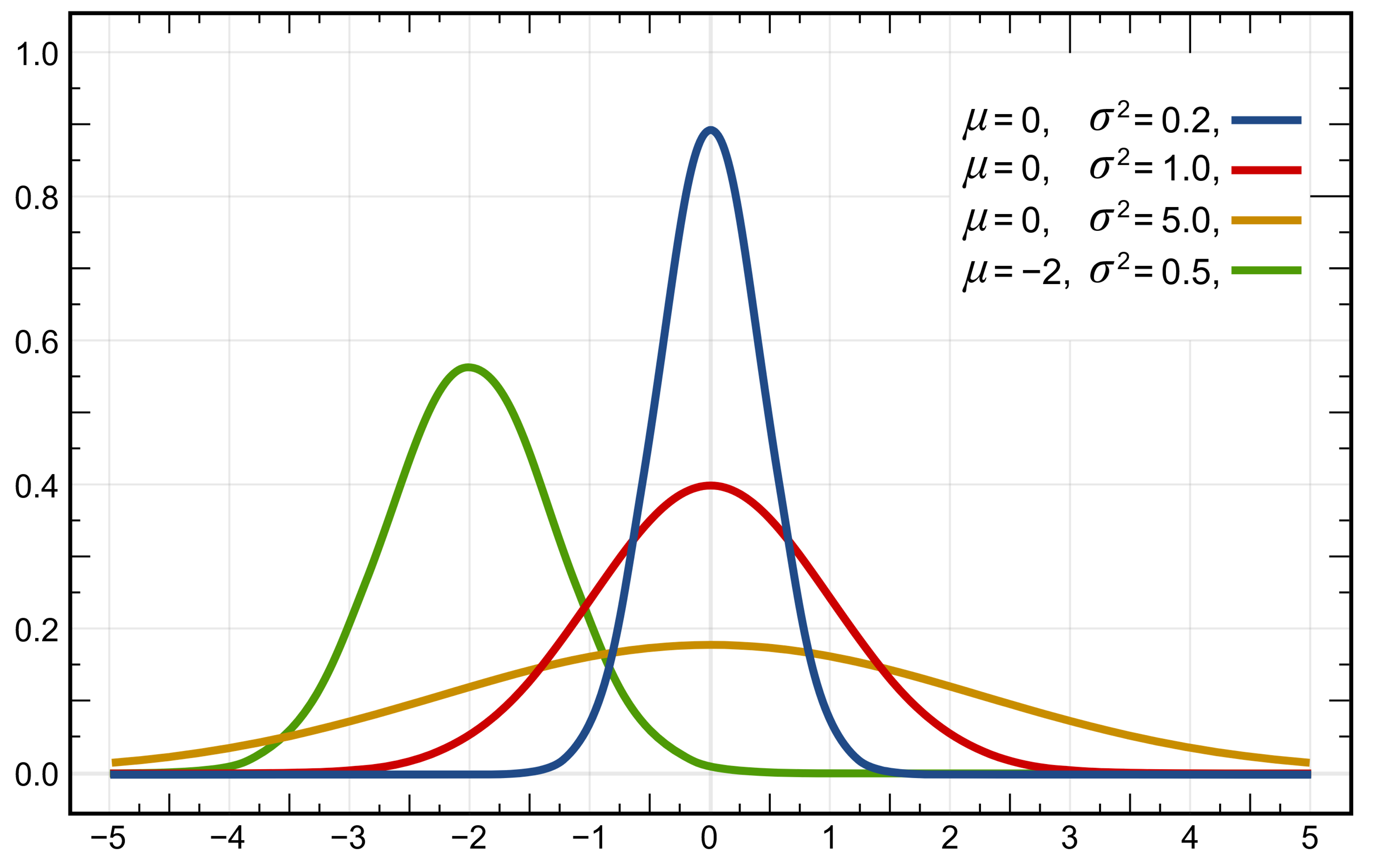
Unlike the uniform distribution, the Gaussian distribution is extremely prevalent in nature. Heights, lengths, weights, temperatures, and many more measures of natural items typically show a Gaussian distribution. In this distribution, numbers close to the mean (typically represented by μ) are most likely to be chosen. The standard deviation (typically represented by σ) describes how concentrated or spread out the odds are around the mean.

Aesthetically, Gaussian distributions are good for values that should be approximately the same, but with some outliers for variety:

When the standard deviation is high, Gaussian distributions can produce somewhat erratic results with extreme outliers. Note that Gaussian distributions do not have a min or max, so ocassionally it can be useful to bound them.

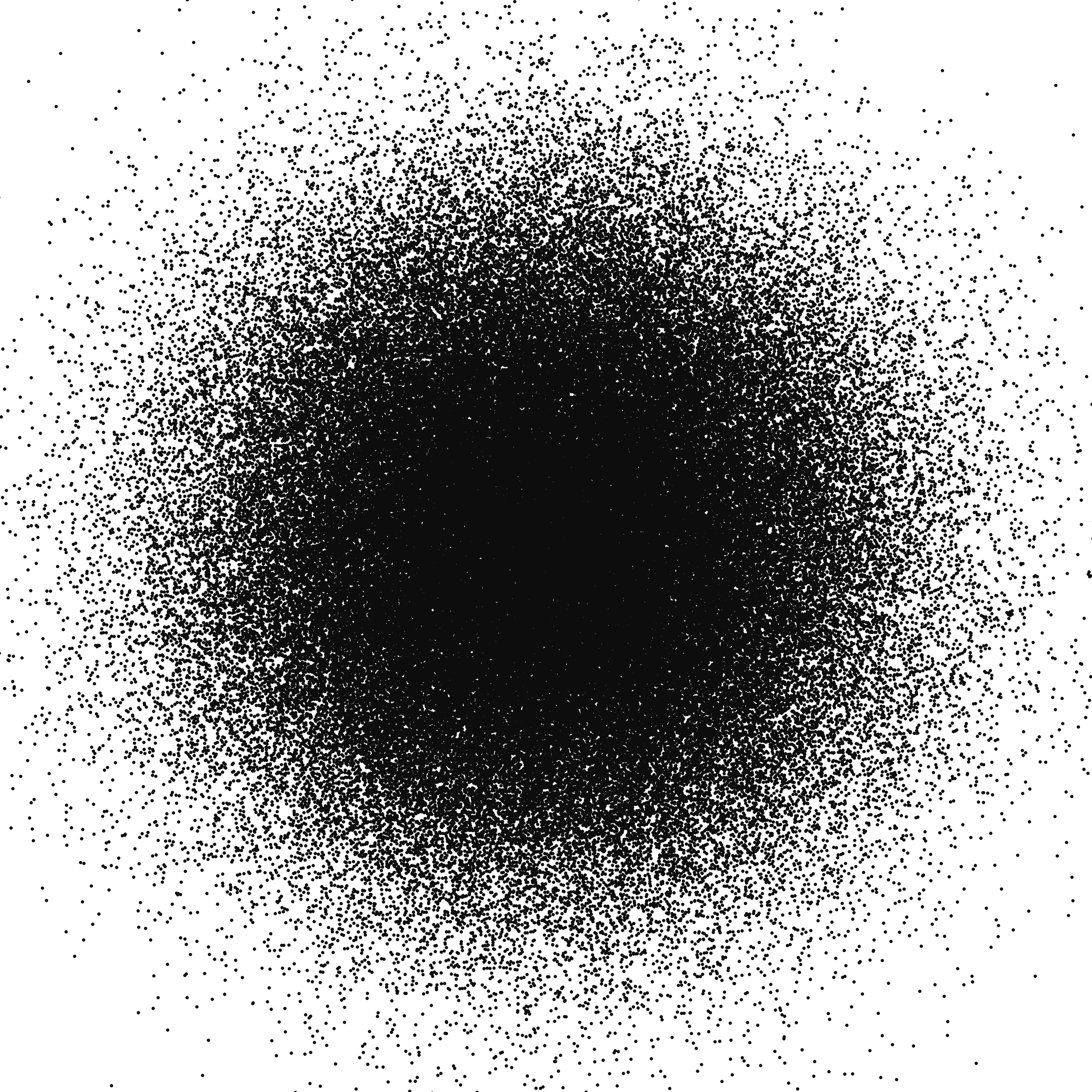
When used for x and y coordinates, this distribution produces a cloud:

If you're using Processing, the randomGaussian() function will use a Gaussian distribution with a mean of 0 and a standard deviation of 1. To change the mean, simply add the desired mean to the result of randomGaussian(). To change the standard deviation, multiply the result.

This is the distribution that I use most frequently.

Power Law Distribution

Power law distributions are exponentially skewed towards a defined minimum. The probability of a number being randomly selected exponentially decreases as the number gets larger:

The Pareto distribution is perhaps the most commonly used power law distribution. Examples of this distribution in real life include the population of cities (many small cities, few very large cities) and the wealth of individuals (many poor individuals, few very rich).

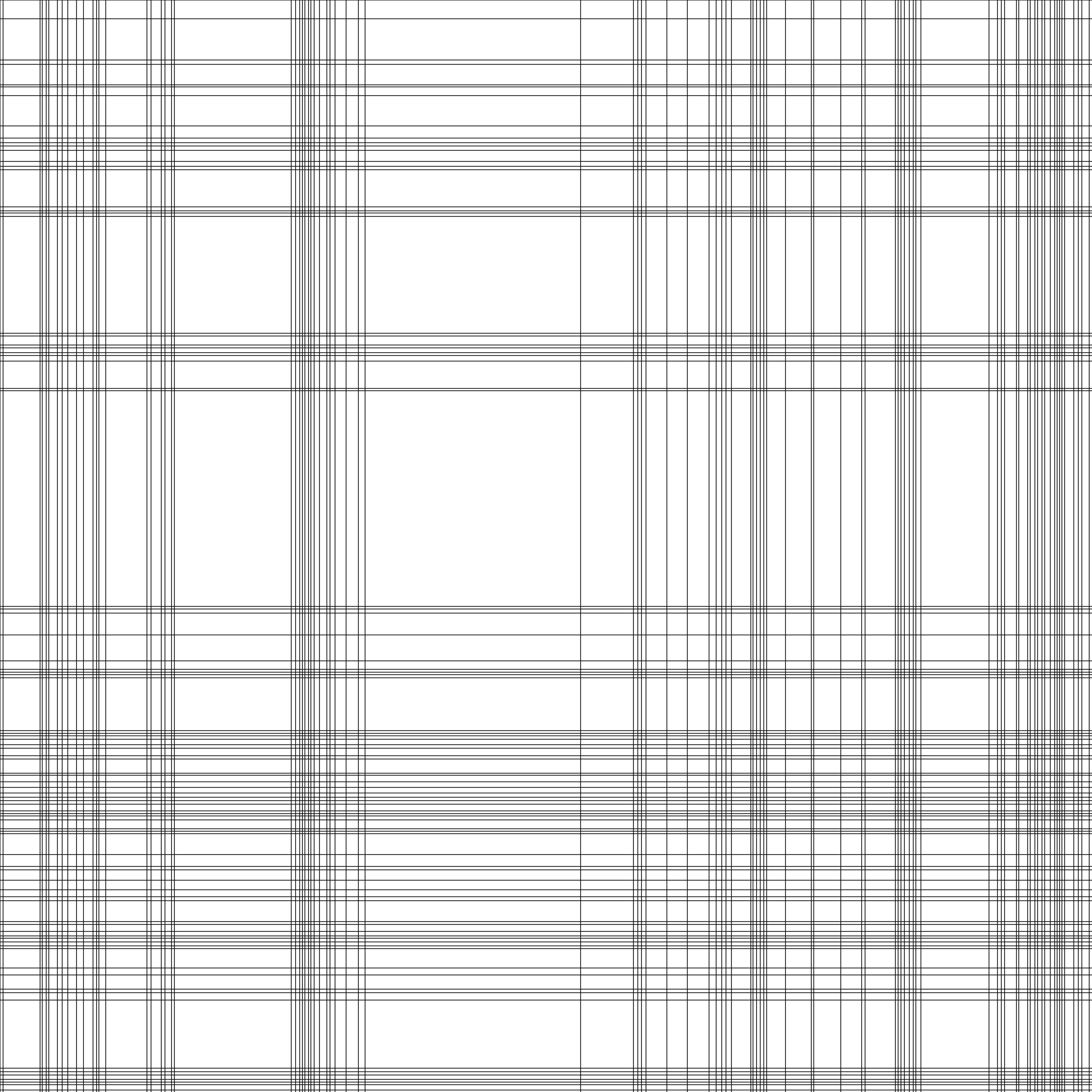
Aesthetically, the Pareto distribution is useful for achieving a balance of different sized objects. The range of sizes can be very large, but you are likely to get very few large objects:

For example, in my Community series of works, I used a pseudo-Pareto distribution to choose the length and width of polygons. Note that there are many tiny polygons, but very few large polygons. The number of small, medium, and large objects is well-balanced.